This part of a three part series on STL decomposition focuses on a sketch of the algorithm. It is not a rigorous treatment, but hopefully thorough enough to provide a mathematical understanding of how the various hyperparameters affect the decomposition. This post is a bit heavy on the mathematics. For an introduction to STL, please look at Part I

STL (Seasonal Trend decomposition using Loess) was developed by Cleveland et al. Journal of Official Statistics 6 No. 1 pp 3-33 1990. The core idea is that a time series can be decomposed into three components: seasonal, trend and remainder (\(Y_\nu = T_\nu + S_\nu + R_\nu\)) for \(\nu = 1\) to \(N\) measured data points. The algorithmic details is not commonly discussed in time series texts in part because unlike other methods, there is no notion of a loss function to be minimized. This is because the notional of seasonal variation is always intrinsically ambiguous: whether the temporal variation should be considered Seasonal, Trend, or Remainder is, to a degree, a matter of opinion and determined by choice of model and model parameters. This is true in STL as well as any seasonal variational approach.

Key to the STL approach is Loess (LOcal regrESSion) smoothing. For a set of measurements \(y_i\), and \(x_i\), Loess provides smooth estimate \(g(x)\) for \(y\) at all values of \(x\), not just at values \(x_i\) for which \(y\) has been measured. To calculate \(g\), a positive integer \(q\) is chosen. A larger \(q\), yields greater smoothing. The \(q\) values of \(x_i\) that are closes to \(x\) are selected and each is weighted by how far it is from \(x\). The weight is determined as \(v_i = W( | x_i−x |\)) where \(W\) is the tricube weight function and \(\lambda_q (x)\) is the distance from the \(q^{th}\) farthest point (for \(q < N\). If \(q >= N\), additional scale terms must be used). A polynomial of degree \(d\) (typically one or two) is fit to the selected \((x_i,y_i)\) with weights \(v_i\). In addition, it is possible to have a set of robustness weights \(\rho_i\) for each data point \((x_i, y_i)\). These weights allow for some data points to be considered more heavily in the regression. If robustness weights exist, use weights \(\rho_i v_i\). For STL, selection of smoothing parameters \(q\) and to a lesser extent \(d\) are a key model choice.

Algorithmic sketch

The goal is to separate a time series \(Y_\nu\) for \(\nu = 1\) to \(N\) into \(Y_\nu = T_\nu + S_\nu + R_\nu\), trend, seasonal and remainder components. This is done through two loops. In the outer loop, robustness weights are assigned to each data point depending on the size of the remainder. This allows for reducing or eliminating the effects of outliers. The inner loop interatively updates the trend and seasonal components. This is done by subtracting the current estimate of the trend from the raw series. The time series is then partition into cycle-subseries (e.g. if it is monthly data with a yearly season, then there will be 12 cycle subseries: all Januarys will be one TS, all February a second, etc.). The cycle-subseries are loess smoothed and then passed thorough a low-pass filter. The seasonal components are the smoothed cycle-subseries minus the result from the low-pass filter. The seasonal components are subtracted from the raw data. The result is loess smoothed, which becomes the trend. What is left is the remainder. In the outline below, the notation follows the Cleveland paper.

1. Initialize trend as \(T_\nu^{(0)} = 0\) and \(R_\nu^{(0)}=0\)
2. Outer loop - Calculate robustness weights. Run \(n_{(o)}\) times
   • Calculate \(R_\nu\)
   • Calculate robustness weights \(\rho_\nu = B( | R_\nu |/h)\) where \(h = 6 ∗ median( | R_\nu |)\) and \(B\) is the bi-square weight function [1]
   • On initial loop, \(\rho_\nu\) = 1
3. Inner loop - Iteratively calculate trend and seasonal terms. Run \(n_{(i)}\) times
   • Detrend: \(Y_\nu − T_\nu^{(k)}\) where \(k\) is the loop number. If the observed value \(Y_\nu\) is missing, then the detrended term is also missing
   • Cycle-subseries smoothing: The detrended time series is broken into cycle-subseries. For example, monthly data with a periodicity of twelve months would yield twelve cycle-subseries, one of which would be all of the months of January. Each cycle-subseries is then loess smoothed with \(q = n_(s)\) and \(d=1\). The smoothed values yield a temporary seasonal time series \(C^{k+1}\).
   • Low-pass filter: The low pass filter on \(C^{k+1}\) yields \(L^{k+1}\). This filter is the application of two moving averages of lag equal to three followed by loess filtering with \(q = n_{(l)}\) and \(d=1\). \(n_{(l)}\) is defaulted the smallest odd integer greater than the period (e.g. 13 for monthly data). The output of the low-pass filter is \(L^{k+1}\)
   • Detrending of smoothed cycle-subseries: \(S^{k+1} = C^{k+1} − L^{k+1}\). This is the \(k+1\)-th estimate of seasonal component. Importantly, the low-pass filter causes this seasonal time series to average to be nearly zero.
   • Deseasonalizing: \(Y − S^{k+1}\)
   • Trend smoothing: Loess smooth the deseasonalized time series with \(q=n_{(t)}\). Results in \(T^{k+1}\), the \(k+1\)-th estimate of the trend component.

Model parameters

There are six major parameters in the model. The parameter names used in the stlplus package are in parentheses.

• \(n_{(p)}\) (n.p) = the periodicity of the seasonality.
• \(n_{(i)}\) (inner) = number of cycles through the inner loop. Number of cycles should be large enough to reach convergence, which is typically only two or three. When multiple outer cycles, the number of inner cycles can be smaller as they do not necessarily help get overall convergence. The default value in stlplus is 2.
• \(n_{(o)}\) (outer) = number of cycles through the outer loop. More cycles here reduce the affect of outliers. For most situations this can be quite small (even 0 if there are no significant outliers). The default value in stlplus is 1.
• \(n_{(l)}\) (l.window) = the span in lags for the low-pass filter. Almost always taken as the least odd integer greater than or equal to \(n(p)\)
• \(n_{(s)}\) (s.window) = smoothing parameter for the seasonal filter. As \(n_{(s)}\) increases, each cycle subseries becomes smoother. This is one of the parameters with the most freedom of choice from the modeler. It looks like it can become a question of what the modeler believes is changes in seasonal behavior versus aberrant behavior. In stlplus, s.window can accept the keyword “periodic” instead. The package notes say this makes smoothing “effectively replaced by taking the mean.”
• \(n_{(t)}\) (t.window) = smoothing parameter of the trend behavior. As this increases, the trend is increasingly smoothed. The authors recommend “consider [the trend] to be a component whose estimation is needed to form an estimate of the seasonal.” If more careful trend modeling is needed, they recommend first extracting the seasonal, then model the sum of \(T_\nu + R_\nu\). The default value comes from analysis by Cleveland et al. as a relationship between the \(n_{(p)}\) and \(n_{(s)}\). This default keeps it roughly from 1.5 to 2 times \(n_{(p)}\). I have never found any need to adjust this.

In addition to these six primary parameters, the degree of the loess smoothing can be changed, though this is hardly ever needed. The default is typically \(d\) = 1 for all the smoothing. There are more parameters in the stlplus function related to minutia of handling the ends of the time series (such as which cycle-subseries is at the beginning) and some that are related to the computation parameters and (I believe) should not affect the resulting model.

Selecting parameters

Of all of these parameters, the most important for the modeler to consider are \(n_{(p)}\) and \(n_{(s)}\). The decision of which value of \(n_{(p)}\) comes from what seasonal behavior is wanted to be captured. As shown in Part I, traffic has weekly seasonality, but also monthly variation. If multiple seasonalities exist, it is typically best to handle the highest frequency variations first, then aggregate and analyze the slow variations: e.g. find the weekly variation first. Account for that seasonality and then aggregate to monthly data to look at monthly variations.

\(n_{(s)}\) controls the smoothing of the seasonal data. This plays a huge role in determining what variation is considered ‘seasonal’ versus ‘trend’ or ‘remainder.’ The smaller the value, the less smoothing in each cycle-subseries. This causes more of the variation to be captured in the seasonal component. To see this in action, we’ll look again at the traffic data from Part I.

As a reminder, the procedure for performing the stl analysis is

library(stlplus)
weekDays <- c("Su", "M", "Tu","W", "Th", "F", "Sa")

stlDaily <- stlplus(jfkManhattan$Total,t=jfkManhattan$Date,
                    n.p=7, s.window=25,
                    sub.labels=weekDays, sub.start=1)

Plots of the cycle-subseries, using the plot_seasonal function, show how the seasonal term is being smoothed. These plots show each cycle-subseries after subtracting off the trend component and the average value so that each cycle-subseries is centered at zero. The circles in each plot are the data and the line is the result of the seasonal smoothing. The plots below show a range of other values for \(n_{(s)}\):

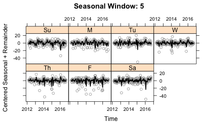
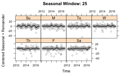
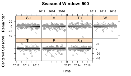
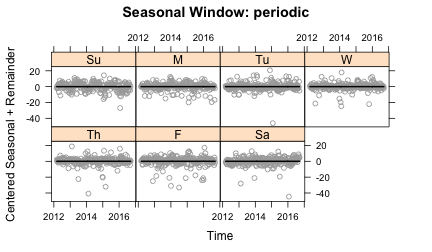
With \(n_{(s)}=5\), there is not enough smoothing to the seasonal component. The line moves too quickly to compensate for changes that should probably be put into the remainder term. \(n_{(s)}=25\) allows for some slow changes in the seasonality, whereas \(n_{(s)}=500\) yields straight lines and \(n_{(s)}=periodic\) gives a constant value. So what is the right answer? This exposes the subjective nature of seasonal decomposition. I personally like capturing some of the variation in seasonality given with \(n_{(s)}=25\). But it certainly wouldn’t be wrong to make a different choice.

Conclusion

I hope this gives at least a bit of a background on how STL works under the hood. The approach I have found best when working with STL is to focus on the \(n_{(s)}\) and \(n_{(p)}\) parameters. \(n_{(p)}\) is determined by what periodicity I am interested in. To choose \(n_{(s)}\), I have to make a series of plots and make the subjective choice of what I want to consider as seasonal.

[1] \(B(u) = (1 - u^2)^2\) for \(0 \le u \le 1\) \(B(u) = 0\) for all other \(u\)